Introduction to Tidyverse : readr, tibbles, tidyr & dplyr

A cheat-sheet walk through

What is Tidyverse?

Tidyverse is a collection of packages for R that are all designed to work together to help users stay organized and efficient throughout their data science projects. The core packages of Tidyverse consist of the following 8 packages:

1. readr: for data import.
2. tidyr: for data tidying.
3. tibble: for tibbles, a modern re-imagining of data frames.
4. dplyr: for data manipulation.
5. stringr: for strings.
6. ggplot2: for data visualisation.
7. purrr: for functional programming.
8. forcats: for dealing factors.

See more on the tidyverse site.

Tidyverse and Rstudio have put out extremely helpful cheat-sheets for each of these packages. Each cheat-sheet contains a lot of information and can appear a bit daunting. The aim of this post is to walk through a few commands from each section of the cheat-sheets in order to get a grasp of the tools and to then have the cheat-sheets as a reference. I will cover readr, tibbles, tidyr, & dplyr, the necessary packages for getting started.

Relevant Cheat-Sheets :

Data Import :: Cheat Sheet (readr, tibble, tidyr) ; Download Here

Data Transformation with dplyr :: Cheat Sheet ; Download Here

Data Import -Page 1-

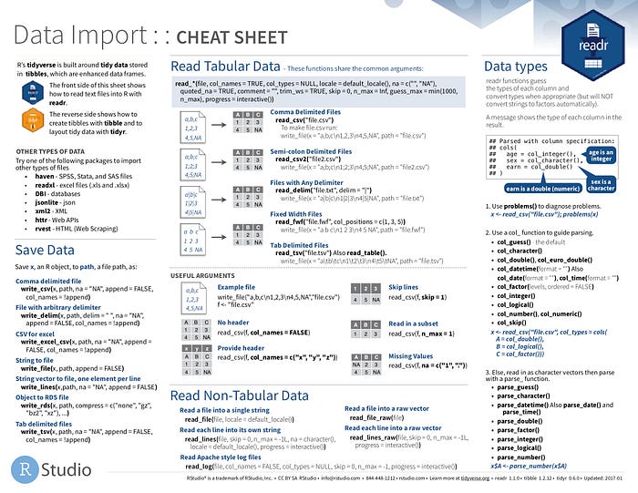
What we’ll cover:

Read Tabular Data: read_csv() , read_excel() -- (via “readxl” package)

Data Types: col_types = , col_double() , col_integer() , col_factor(levels, ordered = FALSE) , parse_integer()

Read Tabular Data

'read_csv( )' , ‘read_excel( )'

I am going to assume that anyone reading this tutorial will be primarily working with tabular data and more specifically CSV’s or Excel Files. For that reason I am only going to touch on these two examples.

note: Tabular data just means represented by a table [i.e. Rows and Columns], this could also be reffered to as rectangular data etc..

What is a Delimiter?
A delimeter is simply a character that seperates different portions of text:

[dog cat mouse goat] <- Here the delimiter would simply be a “ ” ( space) but that wouldn’t work well if you had strings that had spaces in them right.

[dog,cat,mouse,goat] <- Here the delimiter would be a “,” (comma). We need to specify the delimiter in order for the computer to read basic text files into a rectangular format.

What is a CSV?
A CSV or “comma-seperated values” is essentially the same thing as saying a comma delimited file.

Now lets look at some of the examples on the cheat sheet. Lets start out by making the CSV file they suggest:

note: you should see in each example the write_file() function that are quickly making the example files. you can see that the “x =” argument is the text within the file. so ”a,b,c\n1,2,3\n4,5,NA” is an example of what a raw csv file would look like if you were to open it up in a text editor.

# We have to start with loading the tidyverse 
library(tidyverse)
write_file(x=”a,b,c\n1,2,3\n4,5,NA”, path = “file.csv”)
# okay now, lets read it back into our enviorment
tibble_1 <- read_csv(“file.csv”)
tibble_1 

Okay great, thats simple enough right. Now let's try with an excel document. I am using a titanic excel sheet that I have but you can use whatever you want, just make sure you are in the same location as the file or specify the address. For excel documents we actually need to load another package called “readxl”:

install.packages(readxl)
library(readxl)
read_excel(“TitanicList.xlsx”, sheet = 1)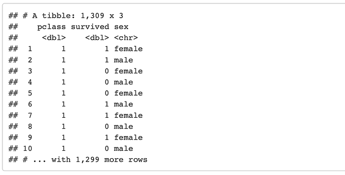

This is pretty self explanatory, so I don't want to spend too much time on it. However the one important thing to recognize is the “sheet = “ argument, as excel files often contain different sheets so you will probably use this many times to specify which sheet you want to read in.

Data Types

col_types = , col_double() , col_integer() , col_factor(levels, ordered = FALSE) , parse_integer()

What is Parsing?

In this context parsing is simply labeling each column as a specific datatype. This is something that readr will try to do automatically .

Let's make a new file.csv to practice with; giving each column a different type.

write_file(x=”a,b,c,d\n1,T,3,dog\n4,FALSE,NA,cat\n6,F,5,mouse\n18,TRUE,3,moose”, path = “file2.csv”)
read_csv(“file2.csv”)

You can see how readr will tell you how it parsed each column. Notice it also changed our ‘column b’ values from ‘T’ to ‘TRUE’, and ‘F’ to ‘FALSE’ to make them all the same format.

'col_types ='

Now lets try parsing manually using the col_types = argument. This way we can specify that column ‘d’ is actually a factor.

x <- read_csv(“file2.csv”, col_types = cols(a = col_double(),b = col_logical(),c = col_integer(), d = col_factor(c(“dog”, “cat”, “moose”, “mouse”), ordered = FALSE)))
# and now lets take a look:
x

Okay great, the one thing to note is that if you parse into a factor it will force you to specify the levels and whether or not they are ordered.

Parsing after reading the file
Unless you are working with files that you are farmiliar with it might be best to parse columns after loading the data. This way you can actually explore the data and see what your working with. for an examlpe lets change column a to an integer type instead of a double.

x$a <- parse_integer(x$a)
x

Great, now you can see that column a is of the type integer. You should note here that you have to reassign column here if you just ranparse_integer(x$a) you would simply return the parsed column, but it would not permentely change the ‘x’ tibble.

Cheat-Sheet 1 : Page 2 (Tibbles & Tidyr)

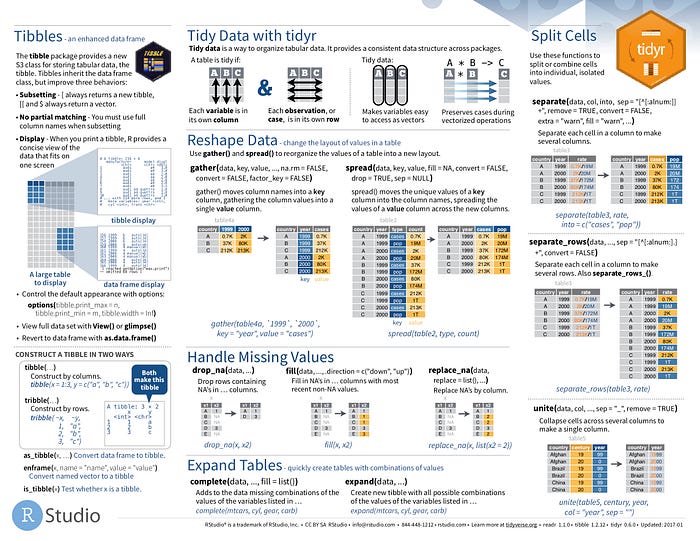
What we’ll cover:
Tibbles : tibble() , as_tibble()
Reshape Data : gather() , spread()
Handle Missing Values: drop_na() , fill() , replace_na()
Expand Tables: expand()
Split Cells: seperate() , unite()

Tibbles

What is a tibble?
A tibble is effectively the exact same thing as a dataframe with more enforcements. These enforcements keep data consistent and ensure compatibility and efficiency throughout a data-science project. So whats an example of these enforcements?

You have already seen how if you want to parse a column as a factor datatype you are forced to specify the levels of the factor as well as whether or not they are ordered. This is not required in a base R data.frame.

Let’s start by making our own tibble. lets make the same table as file2.

y <- tibble(a = c(1,4,6,18), b = c(T,FALSE,F,TRUE), c = c(3, NA, 5, 3), d = c(“dog”,”cat”,”mouse”,”moose”))
y
class(y)

You can see that R will still view its class as a ‘data.frame’ in addition to ‘tbl’ and ‘tbl_df’.

Now lets say we want to convert a dataframe to a tibble. Lets first make the same table as a dataframe and see what differences we notice.

df <- data.frame(a = c(1,4,6,18), b = c(T,FALSE,F,TRUE), c = c(3, NA, 5, 3), d = c(“dog”,”cat”,”mouse”,”moose”))
df
class(df)

Okay so theres the dataframe. What differences do you notice? One; it doesnt list the dimensions of the table, and two it doesnt specify the datatypes of each column.

Now we simply use as_tibble() to convert the dataframe to a tibble.

df <- as_tibble(df)
class(df)

And it’s that simple.

Reshape Data

'gather( )' , ‘spread( )'

Both of the functions seen in this section are represented very clearly in the cheat-sheet. They are also exactly opposites of one another. I would encourage you too look at the images shown in the cheat-sheet to get an idea of what they do, then practice it with me.

lets first create table4a as seen on the cheat-sheet.

table4a <- tibble(country = c(“A”,”B”,”C”), “1999” = c(“0.7K”,”37K”,”212K”), “2000” = c(“2K”,”80K”,”213K”))
table4a

Okay great, So now what if we instead wanted to have ‘year’ be a variable or column. This is where the gather() function comes into play. Let's give it a shot.

table <- gather(table, `1999`,`2000`, key = “year”, value = “cases”)
table

And it's that simple. Now you can use the year as a factor that you could filter by.

okay now lets go ahead and try to do the exact opposite with the spread() function:

spread(table, year, cases)

Boom back to the original. Try to think of some other use-cases for these functions. Think about dimensionality and when it might be better to have fewer or greater number of variables.

Handling Missing Values

'drop_na( )' , ‘fill( )' , ‘replace_na( )'

What is Imputation?
Imputation is the process of filling in missing data, and I feel it necessary to strike fear into doing anything with missing values without understanding the implications and what options you might have.
Here is a great post about imputation that is definitely worth checking out.
“How to Handle Missing Data” by Alvira Swalin

Here we have three different options:
1. removing any rows containing NA’s; drop_na()
2. Fill in NA’s via the columns most recent non-NA valu; fill()
3. Replace NA’s by the colum; replace_na()

Lets start by making the example tibble:

table <- tibble(x1= c(“A”,”B”,”C”, “D”, “E”), x2 = c(1,NA,NA,3,NA))
table

So, we have a tibble with 2 columns of 5 rows, with some NA’s mixed into the second column.

1. Removing any rows containing NA’s with drop_na(data, …)

drop_na(table)

So what happened? It looks like with the drop_na() it will simply remove any row that has an NA in it. This is obviously an easy way to lose a lot of your data, so be careful.

2. Fill in NA’s with the columns most recent non-NA value with fill(data, …, .direction = c(“down”, “up”))

fill(table, x2)

Another simple answer, which should also be used with caution. You should note that the ‘direction = ‘ argument will default to “up” meaning it will fill the NA with the data above it.

3. Replace NA’s by the column with a specific value withreplace_na(data, replace = list(), …)

replace_na(table, replace = list(x2 = 2))

The only important thing to note here is the fact that. That the ‘replace =’ argument needs to be within list().

Expand Tables

'expand( )'

The expand function creates a new tibble with all possible combinations of the values of variables of interest. What does this really mean?

First we are just pulling out the columns of interest. we will go over this select() function in the next section where we cover the dplyr package.

cars <- select(mtcars, cyl, gear, carb)
cars

Now let’g go ahead and use the expand function to see what we get:

expand(cars, cyl, gear, carb)

So we get a dataframe with every possible combination of these variables. There are 3 different values of ‘cyl’, 3 different values of ‘gear’, and 6 different values of ‘carb’. As you can see there are 54 rows in this dataframe.

3*3*6 = 54.

So what would a use-case be?

what if you simply wanted to get a count of the total number of combinations, you could use this and then count the length of it. Or of you wanted to get the average mpg with each combination of variables you could use this as a reference to make sure you hit address every possible combination.

Split Cells

'separate( )'

These functions are fairly simple, allowing you to split parts of a cell up into multiple cells or vice-versa.

For these examples were going to use table3 a built in table. Lets first take a look at the table.

table3

Okay, so lets say we want to split up the rate into the numerator and the denominator.

separate(data, col, into, sep = “[^[:alnum:]]+”, remove = TRUE, convert = FALSE, extra = “warn”, fill = “warn”, …)

The one thing to note here is the “sep = [^[:alnum:]]+” argument which has a default that will automatically try to separate using any non-alphanumeric values. Otherwise you can use the `sep = ` argument to define the separator?

Bonus Cheat-Sheet: This helps explain pattern matching in R. it will help you understand what [^[:alnum:]]+ actually means. click here for cheat-sheet.

So lets try both the default argument as well as manually specifying the separator:

separate(table3, rate, into = c(“numerator”, “denominator”), sep = “[^[:alnum:]]+”)

Okay perfect, so in this case scenario the default was able to seperate the columns correctly. Now lets just do the same thing specifying the separator.

table3 <- separate(table3, rate, into = c(“numerator”, “denominator”), sep = “/”)
table3

Cool same thing.

‘unite( )’

Now lets go ahead and put the same table back to its orginal state but instead of making the rate a fraction lets make it a ratio with “:” for a separator.

unite(table3, numerator, denominator, col = rate, sep = “:”)

These are obviously functions that will be used quite often. Now lets move on to dplyr.

Data Transformation with dplyr : Page 1

What we’ll cover:

Pipes : %>%
Summarise Cases : summarise() , count() → actually in the Group Cases section.
Group Cases : group_by()
Manipulate Cases : filter() , distinct() , top_n() , arrange() , desc() , add_row()
Manipulate Variables : pull() , select() , mutate () group_by()

Pipes

‘%>%’

Pipes are a very imortant part of dplyr and something that you will probably see and use very often. They have a simple function and are just easy to use. A pipe %>% basically just pushes the data from whatever is before it to the function that is after it.

for example lets just say that we wanted to get the number of rows of mtcars:

mtcars %>% nrow()

Thats it, really simply, but it's a great way to stay organized when you want to do a series of filters, groups, etc, without nesting or making new variables. You will see more examples of this pretty much throughout the rest of this doc.

Summarise Cases

The summarise functions are exactly what they sound like, the cool thing is that you can specify what you want to call each time you summarise. And it returns it in a nice neat table.

‘summarise( )’ , ‘mean( )’ , ‘median( )’ , ‘n_distinct( )’

Lets start by looking at the ‘mpg’ column and the ‘hp’ column and look at the averages, the median value, and the number of distinct cases:

mtcars %>% summarise(mpg_avg = mean(mpg), mpg_median = median(mpg), mpg_ndistint = n_distinct(mpg),
 hp_avg = mean(hp), hp_median = median(hp), hp_ndistint = n_distinct(hp))

Obviously you dont need to look at these side-by-side but the summarize function lets you explore a lot about a data-set with this simple syntax. You can also save it as a tibble and reference it accordingly. There is more all of the nested functions on the next page of the dplyr cheat-sheet.

Group Cases

‘group_by( )’

This is one of my favorite dplyr functions. You can use this function in combination with the summarise function to look at groups of your data. For example lets first group all the cars by the number of cylinders that they have. We can then find the average horse power for each group.

mtcars %>% group_by(cyl) %>%
 summarise(mean(hp))

Great, so the output is a simple table that gives us exactly what we asked for.

‘count( )’

What if we wanted to see how many cars of each group there are…

mtcars %>% group_by(cyl) %>%
 count()

Awesome, This is a super easy and necessary tool for exploring data in R.

Manipulate Cases

`filter( )`

The fiilter function allows you to extract rows from your data that meet certain logical criteria. For example lets say that we want to look at only the cars that are 6 cylinder and above but have less than 150 horse power.

mtcars %>% filter(cyl >= 6 & hp < 150)

Using the logical operators you can subset anything you want here in an easy to read manner, producing a nice clean table as a result. Make sure you are firmiliar with all of the logical and boolean operators shown in the middle of this cheat-sheet page.

`distinct( )`

This will simply give you the distinct or unique values for the variable you select. For example lets check to see the distinct values for ‘gear’.

mtcars%>% distinct(gear)

Another great way to use this tool is to select multiple columns to get the distinct combinations for different variables. For example ask for the distinct combinations of ‘gear’ and ‘hp’.

mtcars %>% distinct(gear, hp)

Lets say we just want to know how many combinations there are:

mtcars %>% distinct(gear, hp) %>%
 count()

I use the distinct() and count() combination all the time when initially exploring a data-set.

'arrange( )'

Let’s say we want to look at the top 10 cars based on their horsepower. Then we want to order them by their displacement (note: displacement in an engine is ~ the volume of the cylinders).

mtcars %>% top_n(10, hp) %>%
 arrange(desc(disp))

Thats pretty self explanatory, the one thing to note is that it will automatically arrange the table in ascending order unless you use the desc() as we did. desc = “descending order”

'add_row( )'

Pretty self explanitory. For this example lets take the table we just made in the example previous and add a new row with some made up information.

mtcars %>% top_n(10, hp) %>%
 arrange(desc(disp)) %>%
 add_row(mpg = 56, cyl = 4, disp = 260, hp= 900)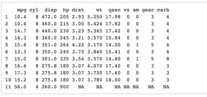

The important thing to note here is that if you miss a column it will still go through and will just fill it in as NA.

Manipulate Variables

'select( )'

The select() function is used to select only the columns that you choose. the output will be a tibble with those selected variables. For example lets say that we want to look at mtcars, but are specifically interested in the ‘qsec’ and the ‘hp’, to remove the noise of the other columns we can make a new dataframe with just those varaibles.

mtcars %>% 
select(qsec, hp) %>%
head()
# just going to show the head to save space

You can also use this function to deselect a column. For example lets say now we want to look at mtcars; and look at every column except ‘qsec’ and ‘hp’. all we have to do is throw the negative sign in front.

mtcars %>% 
select(-qsec, -hp) %>%
head()

Boom, they’re gone.

'mutate( )'

Computing new columns, another must-know function. If you want to make a new column based off other columns, this is the function that you use. Lets go ahead and use the example from the cheatsheet by adding a gallon per mile column.

mtcars %>% mutate(gpm = 1/mpg) %>%
head()

You should see that we added the column ‘gpm’ at the end of the table.

'add_column( )'

Okay now lets go ahead and add our own column, lets say we want to add a column labeling each car into three categorical sizes based off the displacement.
1. small = disp <= 120.8
2. medium = disp > 120.8 & disp <= 326
3. large = disp > 326

First we will use the add_column() function to add the empty column:

# to de-clutter a bit im going to select a couple columns. 
mtcars2 <- mtcars %>% select(disp, hp, qsec) %>% 
 add_column(engine_size = NA)
head(mtcars2)

Now that we have the empty column engine_size, all we have to do is subset out the once that fit in each category and asign the right category.

mtcars2$engine_size[mtcars2$disp <= 120.8] <- “small”
mtcars2$engine_size[mtcars2$disp > 120.8 & mtcars2$disp <= 326] <- “medium”
mtcars2$engine_size[mtcars2$disp > 326] <- “large”
mtcars2 %>% head()

Cool, so now we have a completely new column with a new categorical datatype.

Data Transformation with dplyr : Page 2

What we’ll cover:

Vector Functions : cumsum() , min_rank() , if_else()
Summary Functions: mean() , max(), var()
Row Names: rownames_to_column()
Combine Tables: bind_cols() , bind_rows(), left_join()

Vector Functions

This section shows you a handful of other functions to use with the mutate() to create new columns based on other columns in your table. note: the column of a table is functionally the same thing as a vector. Lets pick out a few of these functions to practice with.

'cumsum( )'

Let's say for example that we are competing in a tag team race across United states. Each team gets 5 cars and one of the race rules is that the total engine displacement for your 5 cars cannot exceed 1000. we can use the cumsum() function to add up the cummulative sum from the ‘disp’ column.

mtcars2 %>% mutate(cum_displacement = cumsum(disp)) %>%
head()

We could then play around with the list, trying to find the most horsepower, or best ‘qsec’ time while keeping the ‘cum_displacement’ under 1000.

note: the one thing to keep in mind here is that the `cum()` function wont reset if you reorder the table, so if you want to play around with the order you have to do it before you mutate the new column.

For example lets say that we wanted to first arrange the cars with the highest hp first and then calculate the cumulative displacement:

mtcars2 %>% arrange(desc(hp)) %>%
 mutate(cum_displacement = cumsum(disp)) %>%
head()

Now we have the cars with the most horse power ‘hp’ but if we just selected these cars we would be in trouble because even after the third car we already have a cummulative displacement over 1000.

‘min_rank( )’

Now lets say that one of the other rules is that we also get scored on how much gas we use in the race; lower the better. Now `mpg` is very important. Lets rank each car against each other by their `mpg`, `hp`, `disp` and their `qsec` .

So for the race we want:

• Low `mpg` (miles/gallon)
• High `hp` (horse-power) notice how we put hp in desc() to get highest
• Low `disp` (displacement)
• Low `qsec` (quarter mile time in seconds)

We can rank them against each other giving a score of 1 as the best. We could then add these scores up where having the lowest overall score as the best car based on these four variables. Lets give it a shot.

# lets first just select our variables of interest.
mtcars3 <- mtcars %>% select(mpg, hp, qsec, disp) %>%
 mutate(mpg_rank = min_rank(desc(mpg)), hp_rank = min_rank(desc(hp)), qsec_rank = min_rank(qsec), disp_rank = min_rank(disp)) %>%
mutate(total_rank = (mpg_rank + hp_rank + qsec_rank + disp_rank )) %>%
 arrange(total_rank) %>%
 # now just for fun lets go ahead and put the cummulative displacement back in there
 mutate(cum_displacement = cumsum(disp)) 
 mtcars3 %>% head()

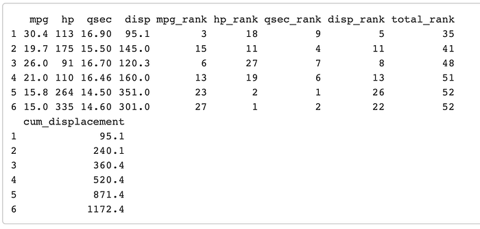
Now look at that the top 5 cars, only add up to 871.4 cummulative displacement so, you could even swap out for a car with a little bit of a larger engine if you wanted to. If this example is confusing, take some time to look at this code to see what each line is doing.

'if_else( )'

Lets say that we want to label the cars good or bad based on their total rank. The mean total_rank is 65.125, so lets jsut say above that is bad and below that is good.

mtcars4 <- mtcars3 %>% mutate(good_bad = if_else(total_rank < 65.125, “good”, “bad” ))
mtcars4 %>% head()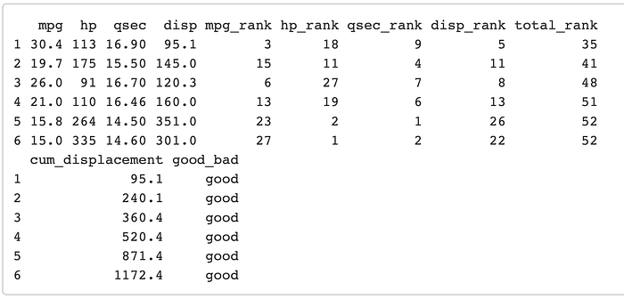

So we made a new column labeling cars good or bad for the race. easy enough.

Summary Functions

We already talked about the summarise() function on the previous page. This section just goes over some of the functions to use inside the summary function.

Some other useful functions to use inside the summarise function:
Center: mean() , median()
Spread: sd() , IQR() , mad()
Range: min() , max() , quantile()
Position: first() , last() , nth()
Count: n() , n_distinct()
Logical: any() , all()

Lets do another quick example. Lets say that we want to compare the good/bad cars by three different things:
1. average qaurter-mile aka ‘qsec’
2. max miles per gallon
3. the variance of the displacement

# first we use the group_by() function:
mtcars4 %>% group_by(good_bad) %>%
 summarise(mean_qsec = mean(qsec), max_mpg = max(mpg), disp_variance = var(disp))

Cool, This is a super handy function that basically makes it easy to pull out any sort of descriptive information in a nice organized table.

Row Names

‘row names_to_column( )’

This is a simple but important function to know. Sometimes you might import data which has the index in the first column, or actual data in the row_names instead of in the first column. The mtcars dataset is actually a perfect example of this. Lets take a look at the dataset as is.

mtcars %>% head()

You can see that the names of the cars are actually the row names rather than the first column in the table. Lets go ahead and put these in column as their own variable.

rownames_to_column(mtcars, var = “car_model”) %>%
head()

One thing to notice here is that you want to set the column name using the var = argument.

Combine Tables

Merging or combining tables is often a pain point and an easy step to make mistakes. You should make sure you know the difference between a left_join, right_join, inner_join and full_join. I am going to skip over it but if you dont know google it, as the distinctions are very important.

'bind_cols( ) ‘

This function is used to simply bind two df’s side-by-side. I would say that the use case for this might be pretty rare, but none-the-less an important one to know. To practice this I am going to split up mtcars into two dataframes and then join them back together.

mtcars1 <- rownames_to_column(mtcars, var = “car_model”) %>%
 select(car_model, mpg, cyl, disp)
mtcars2 <- rownames_to_column(mtcars, var = “car_model”) %>%
 select(car_model, hp, drat, wt, qsec)
mtcars1 %>% head()
mtcars2 %>% head()

head(mtcars1)

head(mtcars2)

You can see that we have two different dataframes here, each with the same number of rows. We know that these rows are going to match up because we just split them up, but in most cases this is where a mistake would be made. So it is really important to know for sure that the two dataframes matchup row-wise.

Now lets go ahead and bind them back together to get our orignal dataset.

mtcars3 <- bind_cols(mtcars1, mtcars2) %>% head()
mtcars3

Notice how we now have two columns that state the car_model, It automatically added a 1 after the second instance of the ‘car_model’ variable, so that no two columns can ever have the same name. In this case, this is a good way to check that they matched up correctly and then we could just deselect that column in the next step.

'bind_rows( )'

This is a much more frequent function in my experience because you use it to add rows of data to a tibble, something that might be done often in a a for-loop for example. I will just do a quick example :

mtcars4 <- bind_rows(mtcars3, mtcars3)
mtcars4

So you can see this function just stacks the two dataframes on top of one another.

'left_join( )'

Were going to practice merging with the left_join function giving us a resulting tibble where every row of the left (first listed) dataframe will be accounted for no matter what. For this example let’s take the two dataframes from the previous example. Lets first take `mtcars1` which has the car_model, mpg, cyl, disp variables. Lets now say that we want to select the top 10 best cars based off of mpg.

mtcars1 <- mtcars1 %>% top_n(10, mpg) 
mtcars1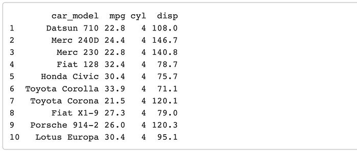

Okay cool so these are the 10 cars with the best mpg. Now lets say that we want to get the rest of the information held in mtcars2 like hp, drat, wt, and the qsec. To do this we are going to join the tables together using a common variable that is unique to every row (hopefully). In this case that unique identifier is the car_model variable.

left_join(mtcars1, mtcars2, by = “car_model”)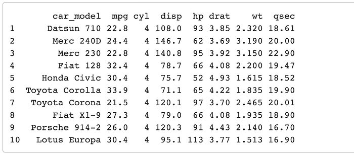

It’s that simple, you just need to make sure that you are using a truly unique identifier, usually an id number or some other form of a primary key.

Wrap-up of dplyr

I am not going to do anymore examples of combining Tables, however I reccomend you familiarize yourself with some of these other more unique functions that might come in hand down the line. dplyr is one of the most popular R packages for good reason. I hope this walk-through gave you a good start to utilize these tools.